Defining a model
Model definitions are specified in a YAML format file, here called definition_input.yml. This
file is parsed and validated by MicroBenthosSchemaValidator.
Upon running with Command: simulate, the validated definition file is written out to
definition.yml.
See the definition file for this tutorial.
Domain
Here we go through the basic steps to define a model. First we have to define a model domain for
a microbial mat or sedimentary system. This is a diffusive system, i.e. the mass transport of
chemical solutes is primarily through physical diffusion. We define the model under the model
key, and specify the domain properties.
2 3 4 5 6 7 8 9 10 | model:
domain:
cls: SedimentDBLDomain
init_params:
cell_size: !unit 50 mum
sediment_length: !unit 10 mm
dbl_length: !unit 2 mm
porosity: 0.6
|
This specifies that the domain should be a SedimentDBLDomain,
with each cell of size 50 micrometers. We specify that the sediment sub-domain is 10 mm long, and
has a 2 mm thick diffusive boundary layer (DBL) on top of it. Additionally, we specify that the
porosity of the sediment domain is 0.6.
Environment
The model environment is a container for various entities that live and interact within the
domain. The environment can contain specifications of
We can specify a solar irradiance within the environment with
13 14 15 16 17 18 19 20 21 22 23 | environment:
irradiance:
cls: Irradiance
init_params:
hours_total: !unit 4h
day_fraction: 0.5
channels:
- name: par
k0: !unit 15.3 1/cm
|
This will render an irradiance source with a diel period (or daylength) of 4 hours with 50% of
the duration being illuminated. Essentially the irradiance source varies in a cosinusoidal
fashion (to approximate solar irradiance) with the specified period. This intensity is at the
surface. However, light propogates variably through a scattering medium like sediments. We can
specify one or more irradiance channels. We specify here that the photosynthetically active
radiation par, usually means 400–700 nm, propagates in the sediment with an exponential
attenuation coefficient of 15.3 per centimeter. As the model clock is incremented, the value of
the surface irradiance varies with a zenith (noon time) value of 100 and dark value of 0. This
“incident” irradiance propagates through the domain according to the channels specified.
Variables
Suppose we want to construct a model where one of the variables we are solving for is the
distribution of oxygen. In the environment we define the variable
26 27 28 29 30 31 32 33 34 35 36 37 38 39 40 41 42 | oxy:
cls: ModelVariable
init_params:
name: oxy
create:
hasOld: true
value: !unit 0.0 mol/m**3
constraints:
top: !unit 230 mumol/l
bottom: !unit 0 mol/l
seed:
profile: linear
# params:
# start: 0.1 mol/l
# stop: 1e-25 mol/l
|
With this block, we have specified a ModelVariable called
oxy. The hasOld: true is necessary to retain the values of the previous time-step during
the simulation evolution. The value is set to 0.0 mol/m**3 here (See using units). For
numerical approximation of the model equations, we have to specify the boundary conditions for
the variables we want to solve for. We specify with constraints here the values at the top
and bottom of the model domains. Optionally, we can specify to seed the initial values of the
variable with a linear profile. Without start and stop conditions given, it will use
the values from the top and bottom constraints. This is only to set the value initially,
i.e. when the model clock is 0. The name entry can be any sympy compatible string, and is
used in string representations of the equation. But the actual key oxy is used in references
of the model path.
Note
Due to current limitations of the solving library fipy, the mesh of the
domain is created in base SI units (meters), and so it is required for now to specify the
variable’s spatial units in meters. MicroBenthos attemps to cast the units to the domain mesh
units internally, but it is better to specify it in the variable creation. All other
parameters can be specified in other SI units and will be converted to the correct units
internally.
Processes
We have only specified a numerical placeholder for the oxygen variable as oxy. In order for
it to behave as a chemical solute diffusing through the model domain, we have to specify the
process that will enable this.
44 45 46 47 48 49 50 51 | D_oxy:
cls: Process
init_params:
expr:
formula: porosity * D0_oxy
params:
D0_oxy: !unit 0.03 cm**2/h
|
Process definitions allow you to write a formula simply as a string, to represent a symbolic
expression that relates various domain variables and parameters. Here we specify the diffusion
coefficient of oxygen D_oxy which is the porosity multiplied by the free diffussion
coefficient D0_oxy. The porosity is 0.6 in the sediment but 1.0 in the DBL, and this
variation will be reflected in the effective diffusion coefficient for oxy at each cell in
the model domain. This is a simple example, but much more complicated dependencies and variations
can be specified symbolically.
Equations
Finally, we need to construct the actual equations we will want to solve. In this simplistic example, we have only defined one variable which should exhibit diffusive transport in the domain . So there will be only one equation for oxygen with only a diffusive and a transient term, as we have not included any other sources or responses to irradiance. That will come in subsequent tutorials, but let’s proceed to build the single equation here.
55 56 57 58 59 | equations:
oxyEqn:
transient: [domain.oxy, 1]
diffusion: [env.D_oxy, 1]
|
We specify an equation named oxyEqn which contains a transient term, pointing to the variable
we want to solve for domain.oxy (this could also be env.oxy), and specify a diffusive
term that takes env.D_oxy as its diffusion coefficient. The second terms is a
multiplicative coefficient for each term in the final equation, here set to 1.
Run it
This creates the equation to solve
Running the model simulation with:
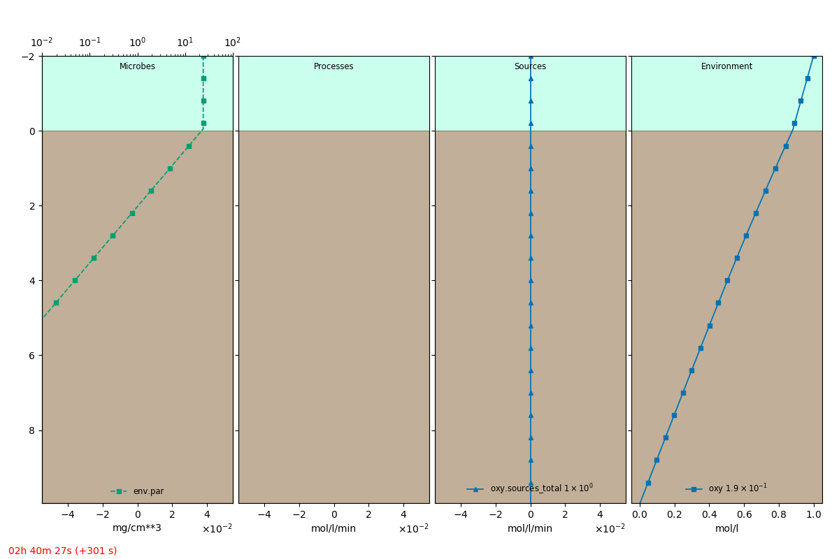
microbenthos -v simulate definition_input.yml --plot --show-eqns
should show the equation in the console and open up a graphical view of the model as it is simulated.
An extracted frame is shown below.
Simulation run
Additionally, we can specify the parameters for the simulation evolution under the main
simulation
key.
63 64 65 66 67 | simulation:
simtime_total: !unit 8h
# simtime_days: 2
simtime_lims: [0.01, 300]
|
We specify with simtime_total that the total time for the simulation run is 8 hours.
Alternatively, one can set simtime_days to a number which will set the simtime_total as the
multiplication of the number with the hours_total of the irradiance source. MicroBenthos
performs adaptive time stepping of the simulation, i.e. increasing the simulation time steps to
larger values when possible and reducing it to smaller time-steps when the equations undergo a lot
of change. The range of the time-steps, usually dependent on the problem being solved, can be set
through simtime_lims, in seconds.
The full definition file is:
# start: model
model:

    domain:
        cls: SedimentDBLDomain
        init_params:
            cell_size: !unit 50 mum
            sediment_length: !unit 10 mm
            dbl_length: !unit 2 mm
            porosity: 0.6
# start: environment
    environment:

        irradiance:
            cls: Irradiance
            init_params:
                hours_total: !unit 4h
                day_fraction: 0.5

                channels:
                    - name: par
                      k0: !unit 15.3 1/cm
# start: oxygen model variable
        oxy:
            cls: ModelVariable
            init_params:
                name: oxy
                create:
                    hasOld: true
                    value: !unit 0.0 mol/m**3

                constraints:
                    top: !unit 230 mumol/l
                    bottom: !unit 0 mol/l

                seed:
                    profile: linear
                    # params:
                    #    start: 0.1 mol/l
                    #    stop: 1e-25 mol/l
# stop: oxygen model variable
        D_oxy:
            cls: Process
            init_params:
                expr:
                    formula: porosity * D0_oxy

                params:
                    D0_oxy: !unit 0.03 cm**2/h
# stop: oxy diffusion
# start: equations
    equations:
        oxyEqn:
            transient: [domain.oxy, 1]

            diffusion: [env.D_oxy, 1]
# stop: equations
# start: simulation
simulation:

    simtime_total: !unit 8h
    # simtime_days: 2
    simtime_lims: [0.01, 300]
# stop: simulation